Introduction

As part of my 2nd-year project at SAE Institute Geneva, I was tasked with building a 3D scene using C++ and OpenGL ES 3.0.

This project was a great opportunity to explore the low-level workings of the GPU. In this blog post, I will present the rendering techniques I used, focusing on key concepts rather than specific implementation details. For a deeper dive, I highly recommend reading LearnOpenGL, which served as my main reference throughout this module.

Engine

Model

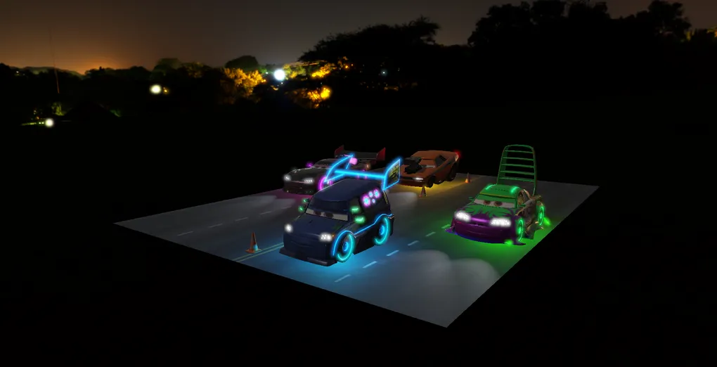
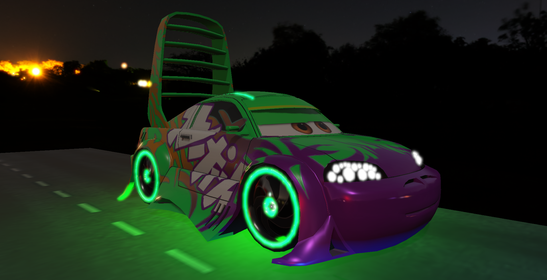
It all starts with importing geometry. I opted for standard Wavefront (.obj) models for their simplicity. For the scene, I chose iconic models from the movie Cars (notably Wingo). However, to achieve a realistic look in my pipeline, I generated compatible textures using PBR Forge since the original models only came with basic textures.

To import the 3D models, I used the Assimp library, which handles generating vertices, indices, and materials.

When loading, I use specific flags to process the data: aiProcess_Triangulate to ensure everything is converted to triangles, and aiProcess_CalcTangentSpace to calculate the tangents needed for Normal Mapping.

Assimp::Importer importer;

const aiScene* scene = importer.ReadFile(
    path,
    aiProcess_Triangulate |
    aiProcess_FlipUVs |
    aiProcess_CalcTangentSpace
);

One important detail: these models aren’t just a single block. They are made up of several distinct Sub-Meshes. That’s why I use a recursive function, ProcessNode, to traverse the entire model hierarchy and extract and store each part of the car independently.

void Model::ProcessNode(const aiNode* node, const aiScene* scene)
{
    for (unsigned int i = 0; i < node->mNumMeshes; i++)
    {
        const aiMesh* mesh = scene->mMeshes[node->mMeshes[i]];
        sub_meshes_.push_back(ProcessMesh(mesh, scene));
    }

    for (unsigned int i = 0; i < node->mNumChildren; i++)
        ProcessNode(node->mChildren[i], scene);
}

The ProcessMesh method takes care of converting Assimp’s data into my own data structures. This is where I grab the positions, normals, and UVs to create my vertices.

Meshes & Vertex Attributes

Once the mesh data is loaded, it needs to be sent to the GPU. To ensure the shader can correctly interpret the raw data, I use a VertexBufferAttribute abstraction that contains all the necessary information to describe a vertex.

struct VertexBufferAttribute {
  GLuint location;
  GLint size;
  GLenum type;
  GLsizei stride;
  size_t offset;
};

This tells OpenGL exactly how my vertex is structured: where to find the position, normal, and UVs, as well as the tangents and bitangents essential for Normal Mapping. I use offsetof to automatically calculate the memory offsets.

constexpr common::VertexBufferAttribute attributes[] = {
    { 0, 3, GL_FLOAT, sizeof(Vertex), offsetof(Vertex, Position) },
    { 1, 3, GL_FLOAT, sizeof(Vertex), offsetof(Vertex, Normal) },
    { 2, 2, GL_FLOAT, sizeof(Vertex), offsetof(Vertex, TexCoords) },
    { 3, 3, GL_FLOAT, sizeof(Vertex), offsetof(Vertex, Tangent) },
    { 4, 3, GL_FLOAT, sizeof(Vertex), offsetof(Vertex, Bitangent) }
};
vertex_input_.BindVertexBuffer(vertex_buffer_, attributes);

Materials & Textures

To load the textures associated with the model, I created a LoadMaterial method. It uses a handy little lambda to check if a texture exists in the .obj file (via Assimp) and automatically loads it into the correct slot of my Material structure.

Material Model::LoadMaterial(const aiMaterial* mat) const
{
    Material m;

    auto LoadTex = [&](const aiTextureType type, common::Texture& dst)
    {
        if (mat->GetTextureCount(type) > 0)
        {
            aiString file;
            mat->GetTexture(type, 0, &file);

            const std::string full = directory_ + file.C_Str();
            dst.Load(full);
        }
    };

    LoadTex(aiTextureType_DIFFUSE,  m.diffuseMap);
    LoadTex(aiTextureType_NORMALS,  m.normalMap);
    LoadTex(aiTextureType_EMISSIVE, m.emissiveMap);
    LoadTex(aiTextureType_SPECULAR, m.metallicMap);
    LoadTex(aiTextureType_SHININESS, m.roughnessMap);
    LoadTex(aiTextureType_AMBIENT, m.aoMap);

    return m;
}

Once the materials are loaded, they need to be sent to the shader. To simplify this, I use the SetTexture method from the Pipeline abstraction.

This method does two important things: it informs the shader which texture unit to use (via a uniform int) and it activates that unit to bind the corresponding texture.

void Pipeline::SetTexture(std::string_view name, const Texture& texture, int texture_unit) {
  SetInt(name.data(), texture_unit);
  glActiveTexture(GL_TEXTURE0 + texture_unit);
  texture.Bind();
}

In the Bind method of the Material class, I use this abstraction to bind all the maps (BaseColor, Normal, Metallic, etc.) in an organized way. I also send booleans so the shader knows if a texture is present or if it should use a default value.

void Bind(common::Pipeline& pipeline) const {
    pipeline.SetTexture("diffuseMap",   diffuseMap,   0);
    pipeline.SetTexture("normalMap",    normalMap,    1);
    pipeline.SetTexture("emissiveMap",  emissiveMap,  2);
    pipeline.SetTexture("metallicMap",  metallicMap,  3);
    pipeline.SetTexture("roughnessMap", roughnessMap, 4);
    pipeline.SetTexture("aoMap",        aoMap,        5);


    pipeline.SetBool("useNormalMap", normalMap.get().texture_name != 0);
    pipeline.SetBool("useMetallicMap", metallicMap.get().texture_name != 0);
    // ...
}

Then the common::Texture class handles the technical side using stb_image.

Normal Mapping

Normal Mapping is used to simulate detail and relief on the car bodywork. The catch is that the normals in a “Normal Map” are defined in Tangent Space (local to the face). To use them in World Space for lighting calculations, we need a transition matrix: the TBN Matrix.

I handle this calculation in the Vertex Shader using the aNormal and aTangent attributes provided by Assimp.

  mat3 normalMatrix = mat3(transpose(inverse(finalModel)));
  vec3 T = normalize(normalMatrix * aTangent);
  vec3 N = normalize(normalMatrix * aNormal);
  T = normalize(T - dot(T, N) * N);
  vec3 B = cross(N, T);

I use the Gram-Schmidt process here to ensure the tangent remains perfectly orthogonal to the normal. Then, I calculate the bitangent using a Cross product.This calculation allows me to transition from Tangent Space to World Space, which is where I perform all my lighting calculations.

Back Face Culling

To optimize rendering, I learned about two culling techniques. The first one is Back-face Culling. It’s a technique that is very quick to implement; it simply tells the GPU to skip drawing the back faces of objects. This reduces the number of triangles to process without impacting the final visual result.

glEnable(GL_CULL_FACE);
glCullFace(GL_BACK);
glFrontFace(GL_CCW); // Définit le sens de lecture des triangles (Counter-Clockwise)

In the image below, our camera is positioned inside the car (Wingo). With Back-Face Culling enabled, all the bodywork faces pointing outward are not rendered. That is why we can see right through the model from the inside.

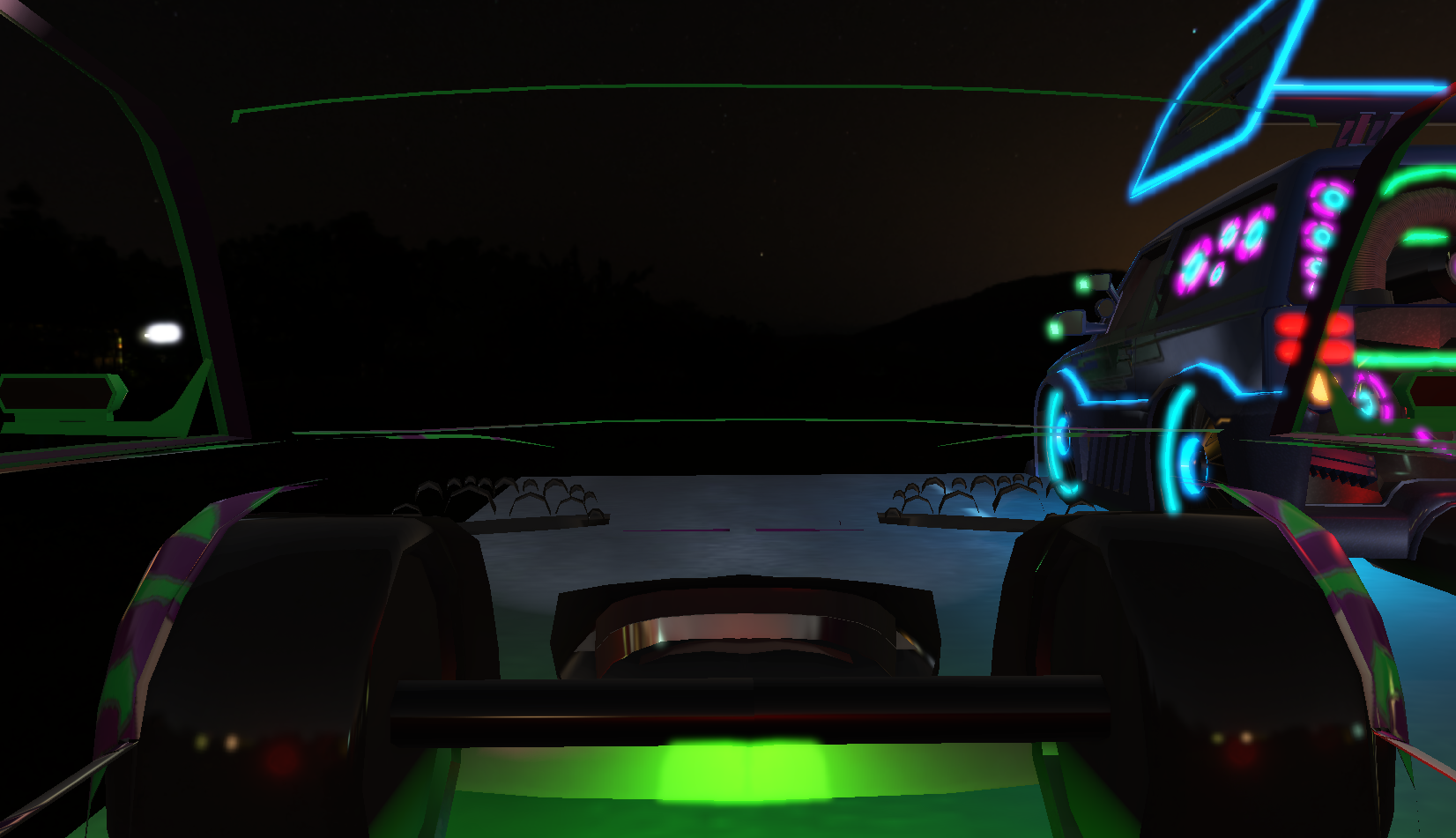
To visually test the concept, we can also switch the mode to Front-Face Culling: in this case, the GPU will only display the interior (the back faces) and hide the car’s exterior.

Frustum Culling

The second technique is Frustum Culling. Unlike Back-face culling, which works at the triangle level, Frustum Culling operates at the model level. The goal is to avoid sending objects to the GPU if they are outside the camera’s field of view.

The field of view is represented by a truncated pyramid (the Frustum) defined by six planes: the Near plane, the Far plane, as well as the top, bottom, left, and right planes.

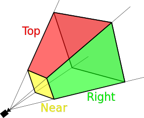
To determine if an object needs to be rendered, I check if it intersects with this viewing volume. Each model has an AABB (Axis-Aligned Bounding Box) member that is pre-calculated during Model::Load.

To put this into practice, I created a very simple Frustum class. It contains the six planes of the view pyramid and features an IsOnFrustum method. This function takes a model’s AABB and its modelMatrix to determine whether the object is visible or not.

class Frustum
{
public:
    void Update(const glm::mat4& viewProjection);
    bool IsOnFrustum(const AABB& box, const glm::mat4& modelMatrix) const;

private:
    std::array<Plane, 6> planes_;
};

I integrated this logic directly into my Camera abstraction. By combining the projection matrix and the view matrix, the camera can generate an updated Frustum every frame.

Frustum Camera::get_frustum() const
{
    Frustum frustum;
    frustum.Update(projection_matrix_ * get_view_matrix());
    return frustum;
}

GPU Instancing

Instancing is another optimization technique. It allows me to render hundreds of identical objects—like my traffic cones—in a single draw call. Instead of sending each cone one by one, I send an array of transformation matrices to the GPU.

To make this work, I have to configure specific vertex attributes. Since a mat4 matrix occupies 4 consecutive slots (locations 5 to 8), I use glVertexAttribDivisor. This tells OpenGL to move to the next matrix only after drawing a complete object, not after every vertex.

void Mesh::SetupInstancing(const common::VertexBuffer& instance_buffer) {
    vertex_input_.Bind();
    instance_buffer.Bind();

    std::size_t vec4Size = sizeof(glm::vec4);
    glEnableVertexAttribArray(5);
    glVertexAttribPointer(5, 4, GL_FLOAT, GL_FALSE, 4 * vec4Size, (void*)0);
    glEnableVertexAttribArray(6);
    glVertexAttribPointer(6, 4, GL_FLOAT, GL_FALSE, 4 * vec4Size, (void*)(1 * vec4Size));
    glEnableVertexAttribArray(7);
    glVertexAttribPointer(7, 4, GL_FLOAT, GL_FALSE, 4 * vec4Size, (void*)(2 * vec4Size));
    glEnableVertexAttribArray(8);
    glVertexAttribPointer(8, 4, GL_FLOAT, GL_FALSE, 4 * vec4Size, (void*)(3 * vec4Size));

    glVertexAttribDivisor(5, 1);
    glVertexAttribDivisor(6, 1);
    glVertexAttribDivisor(7, 1);
    glVertexAttribDivisor(8, 1);
}

On the Shader side, the logic is pretty straightforward. If instancing is enabled, I use the instance matrix received as an attribute (aInstanceMatrix) instead of the standard model matrix. This allows me to position each cone at its own unique location while still using the exact same geometry.

layout (location = 5) in mat4 aInstanceMatrix;
uniform bool useInstancing;

void main() {
    mat4 finalModel = useInstancing ? aInstanceMatrix : model;
    vec4 worldPos = finalModel * vec4(aPos, 1.0);
    
    gl_Position = projection * view * worldPos;
}

Finally, for the actual rendering, I just need to call glDrawElementsInstanced. My Model abstraction takes care of handling this call for all its sub-meshes.

To confirm that instancing was working correctly, I used RenderDoc to inspect the GPU calls. In the screenshot below, you can clearly see the glDrawElementsInstanced call. Instead of drawing a single cone, the GPU generates 4 of them in a single pass using data from my instance buffer (obviously, we can instance way more than just 4 😅).

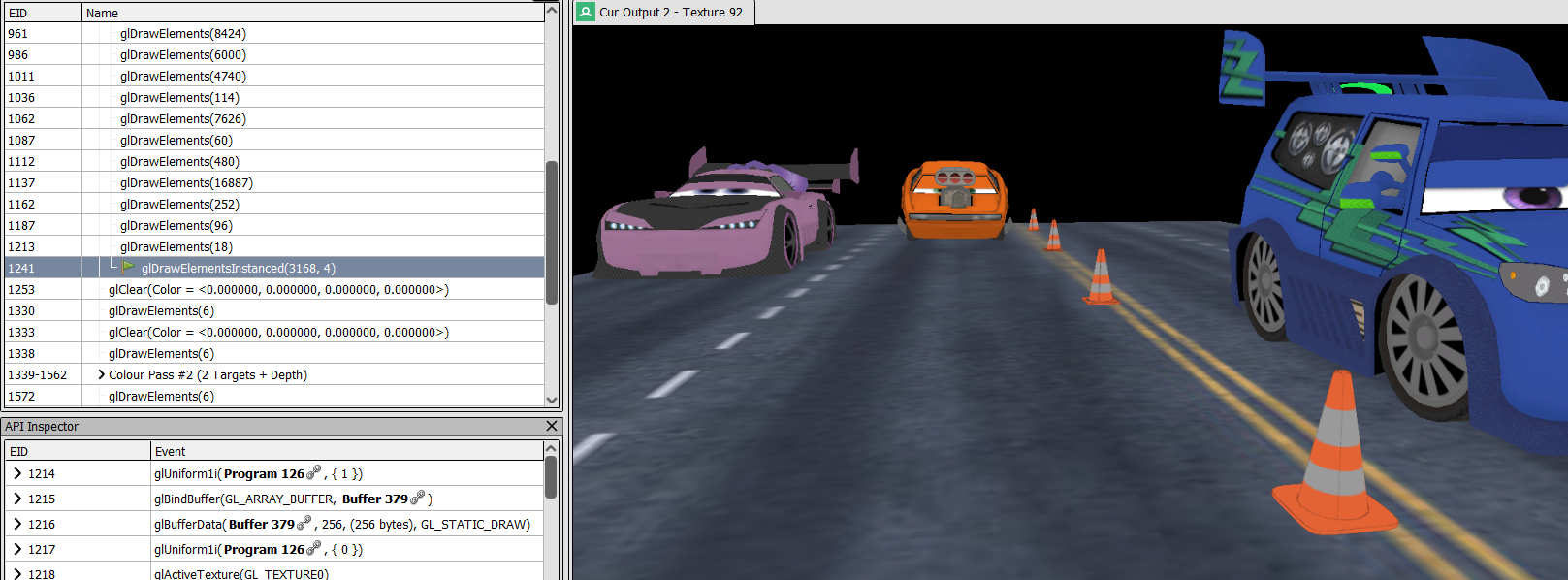
This technique is exactly what keeps the framerate high, even with a scene packed with repetitive objects.

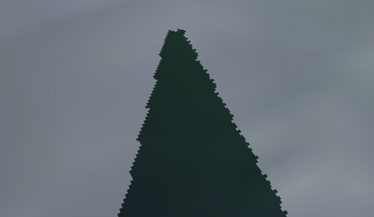
Cubemap

Before tackling the core of the engine, I needed an environment to place my car in. I implemented a Skybox. The principle is simple: draw a giant cube around the camera and apply a texture to each face.

In OpenGL, we use a GL_TEXTURE_CUBE_MAP. It’s a special texture type that treats 6 faces (Right, Left, Top, Bottom, Back, Front) as a single entity.

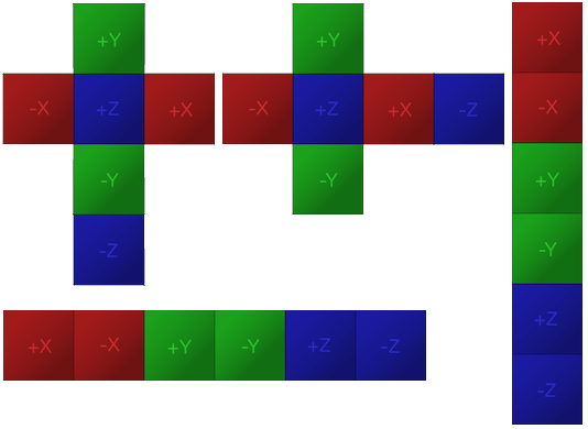
To load this in my common::Texture abstraction, the trick is to loop through the files and use the GL_TEXTURE_CUBE_MAP_POSITIVE_X enum. Since the enums for the 6 faces are sequential in OpenGL, I can simply increment i to target the next face.

glGenTextures(1, &get().texture_name);
glBindTexture(GL_TEXTURE_CUBE_MAP, get().texture_name);

for (size_t i = 0; i < faces.size(); i++) {
    int width, height, channels;
    unsigned char* data = stbi_load(std::string(faces[i]).c_str(), &width, &height, &channels, 0);

    const GLenum format = (channels == 3) ? GL_RGB : GL_RGBA;
    glTexImage2D(GL_TEXTURE_CUBE_MAP_POSITIVE_X + static_cast<GLenum>(i), 0, format, width, height, 0, format, GL_UNSIGNED_BYTE, data);
    stbi_image_free(data);
}

For rendering, there are two important things:

• I remove the translation from the view matrix.
• I change the depth function to GL_LEQUAL to ensure the sky renders at the very back.

void Skybox::Draw(const glm::mat4& view, const glm::mat4& projection)
{
    glDepthFunc(GL_LEQUAL);
    glDisable(GL_CULL_FACE);

    pipeline_.Bind();
    auto viewNoTranslation = glm::mat4(glm::mat3(view));

    pipeline_.SetMat4("view", glm::value_ptr(viewNoTranslation));
    pipeline_.SetMat4("projection", glm::value_ptr(projection));
    pipeline_.SetTexture("skybox", texture_, 0);
    pipeline_.SetFloat("skyboxIntensity", intensity_);

    cube_mesh_.Draw();

    glDepthFunc(GL_LESS);
}

And just like that, we have a Skybox!

Deferred Rendering

Deferred Rendering is the heart of my rendering pipeline. Unlike classic Forward Rendering, where light is calculated for every object as it’s drawn, Deferred Rendering relies on a clear separation between gathering geometric data and the final image calculation. This architecture allowed me to efficiently integrate multiple render passes (Shadows, SSAO, Bloom) without overloading the GPU.

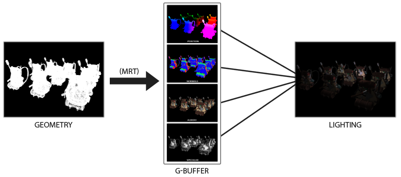
The goal is simple: stop calculating lighting for nothing. In standard rendering, a lot of performance is wasted lighting objects that end up hidden behind others. With the G-Buffer (Geometry Buffer), we flip the logic: we wait until we know exactly which pixels are visible on screen, and we calculate lighting only for those.

Geometry Buffer

The G-Buffer is a set of textures where we store the scene’s geometric information during the “Geometry Pass”. Instead of drawing a final image, we fill several buffers simultaneously:

• Positions
• Normals
• Albedo (BaseColor)
• Emissive
• ARM

To make this work technically, I created a GBuffer class. The most important part is the texture initialization via a createTex lambda. This allows me to cleanly configure MRT (Multiple Render Targets) by attaching each buffer (Position, Normal, Albedo, Emissive) to a specific slot.

auto createTex = [&](GLuint& id, const GLint internal, const GLenum type, const int attach) {
    glGenTextures(1, &id);
    glBindTexture(GL_TEXTURE_2D, id);
    glTexImage2D(GL_TEXTURE_2D, 0, internal, width, height, 0, GL_RGBA, type, NULL);
    glTexParameteri(GL_TEXTURE_2D, GL_TEXTURE_MIN_FILTER, GL_NEAREST);
    glTexParameteri(GL_TEXTURE_2D, GL_TEXTURE_MAG_FILTER, GL_NEAREST);
    glFramebufferTexture2D(GL_FRAMEBUFFER, GL_COLOR_ATTACHMENT0 + attach, GL_TEXTURE_2D, id, 0);
};

createTex(g_position_, GL_RGBA16F, GL_FLOAT, 0);
createTex(g_normal_, GL_RGBA16F, GL_FLOAT, 1);
createTex(g_albedo_, GL_RGBA, GL_UNSIGNED_BYTE, 2);
createTex(g_emissive_, GL_RGBA16F, GL_FLOAT, 3);

Another crucial method is BlitDepthToDefault. Since Deferred Rendering is performed on a simple Quad at the end, we would normally lose the depth information. This function lets me copy the depth buffer from the G-Buffer to the default framebuffer. This prevents the Skybox or other objects from rendering on top of the cars.

void GBuffer::BlitDepthToDefault(const unsigned int width, unsigned int const height) const
{
    glBindFramebuffer(GL_READ_FRAMEBUFFER, g_buffer_);
    glBindFramebuffer(GL_DRAW_FRAMEBUFFER, 0);
    glBlitFramebuffer(0, 0, width_, height_, 0, 0, width, height, GL_DEPTH_BUFFER_BIT, GL_NEAREST);
    glBindFramebuffer(GL_FRAMEBUFFER, 0);
}

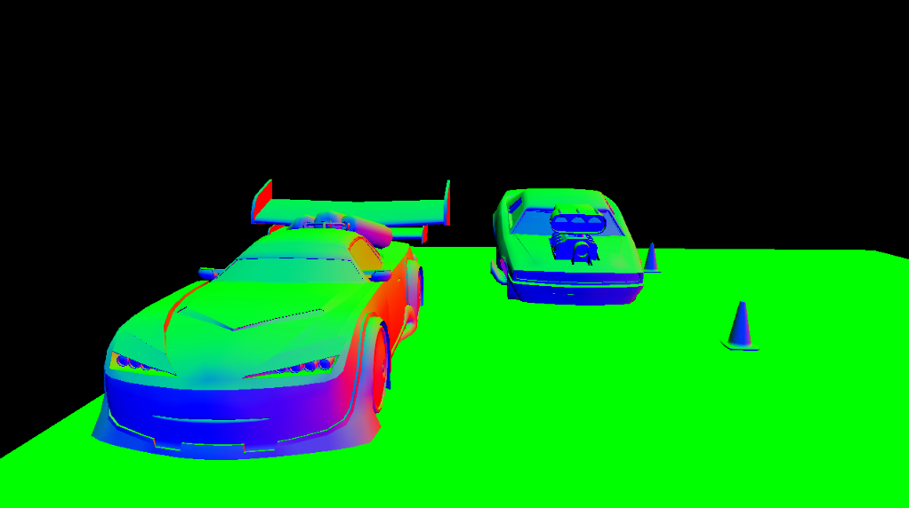
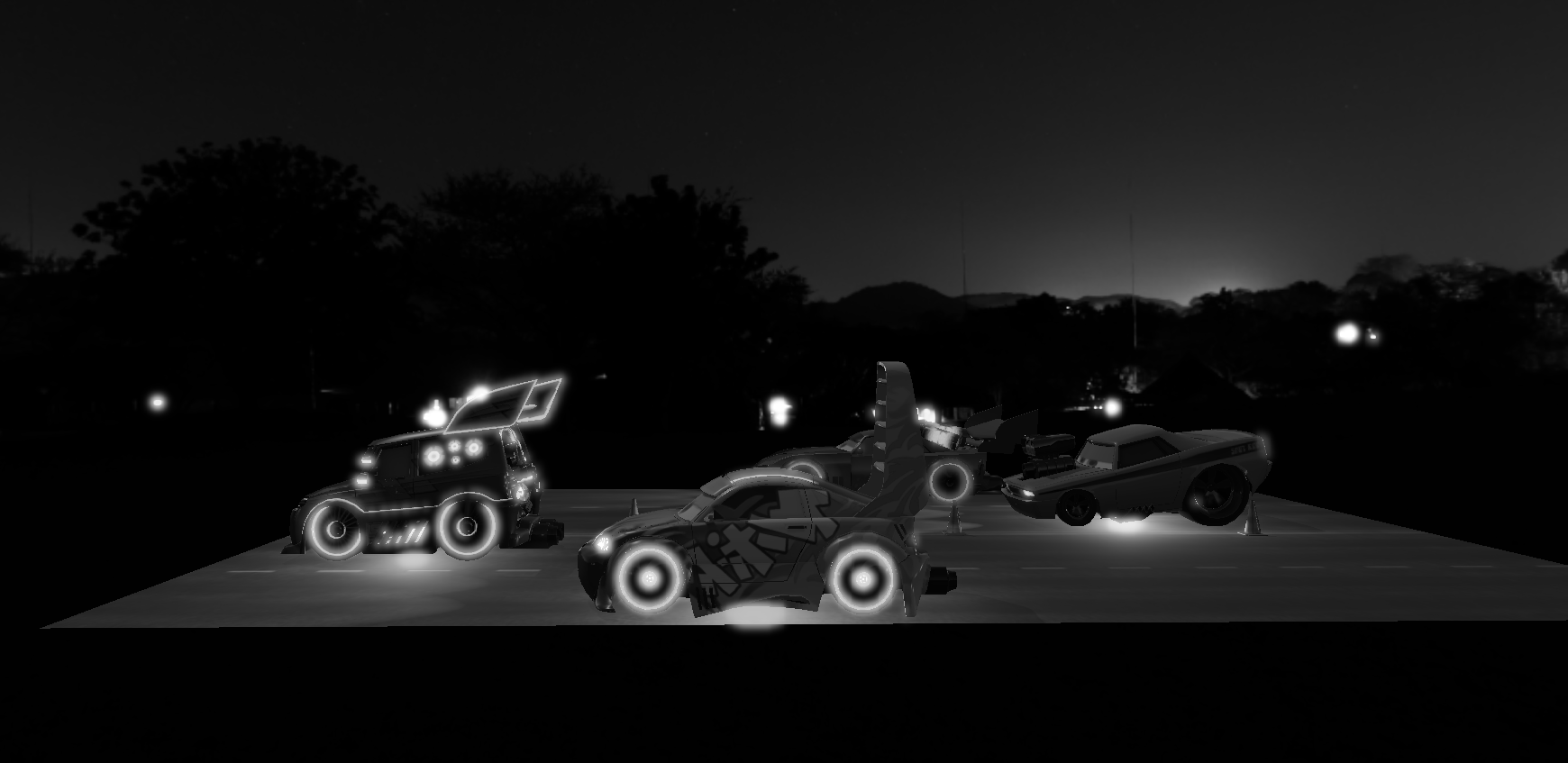
Here is what my various buffers look like when inspected in a RenderDoc capture:

• Positions: Each pixel stores its world coordinates (XYZ).

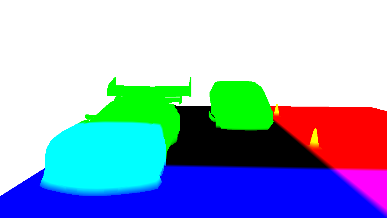
• Normals: The orientation of every surface.

• Albedo: The raw texture colors.

• Emissive: Only the areas that emit light.

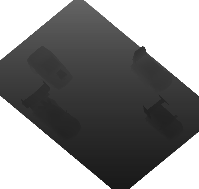
Shadow Pass

Before tackling the G-Buffer, I need to generate a Shadow Map to calculate shadows for my directional light. The idea is to perform a render pass from the light’s perspective to store the scene’s depth in a texture.

In my ShadowMap class, I use an FBO with only a GL_DEPTH_ATTACHMENT. Since I don’t need any color data here, I explicitly disable the read and draw buffers.

glGenFramebuffers(1, &fbo_);
glGenTextures(1, &depth_map_texture_);

glBindTexture(GL_TEXTURE_2D, depth_map_texture_);
glTexImage2D(GL_TEXTURE_2D, 0, GL_DEPTH_COMPONENT24, width_, height_, 0, GL_DEPTH_COMPONENT, GL_UNSIGNED_INT, NULL);

glTexParameteri(GL_TEXTURE_2D, GL_TEXTURE_MIN_FILTER, GL_NEAREST);
glTexParameteri(GL_TEXTURE_2D, GL_TEXTURE_MAG_FILTER, GL_NEAREST);
glTexParameteri(GL_TEXTURE_2D, GL_TEXTURE_WRAP_S, GL_CLAMP_TO_EDGE);
glTexParameteri(GL_TEXTURE_2D, GL_TEXTURE_WRAP_T, GL_CLAMP_TO_EDGE);

glBindFramebuffer(GL_FRAMEBUFFER, fbo_);
glFramebufferTexture2D(GL_FRAMEBUFFER, GL_DEPTH_ATTACHMENT, GL_TEXTURE_2D, depth_map_texture_, 0);

constexpr GLenum drawBuffers[] = { GL_NONE };
glDrawBuffers(1, drawBuffers);
glReadBuffer(GL_NONE);

glBindFramebuffer(GL_FRAMEBUFFER, 0);

For a directional light, I use an orthographic projection. The lightSpaceMatrix combines this projection with a view positioned facing the scene.

const glm::mat4 lightProjection = glm::ortho(-orthoSize, orthoSize, -orthoSize, orthoSize, zNear, zFar);
const glm::mat4 lightView = glm::lookAt(lightPos, target, glm::vec3(0.0f, 1.0f, 0.0f));
light_space_matrix_ = lightProjection * lightView;

The shader is minimal. It transforms vertices directly into light space. No need for a complex fragment shader; OpenGL handles depth writing automatically.

void main() {
    mat4 finalModel = useInstancing ? aInstanceMatrix : model;
    gl_Position = lightSpaceMatrix * finalModel * vec4(aPos, 1.0);
}

Here is what the depth texture looks like when captured from the light source:

Once the depth texture is generated, I handle the shadow calculation in my main fragment shader, deferred_lit.frag. To avoid Shadow Acne (black stripes caused by calculation imprecision), I apply a standard Bias and a Normal Bias that depends on the face’s angle relative to the light.

float ShadowCalculation(vec4 fragPosLightSpace, vec3 normal, vec3 fragPos) {
    vec3 projCoords = fragPosLightSpace.xyz / fragPosLightSpace.w;
    projCoords = projCoords * 0.5 + 0.5;

    if(projCoords.z > 1.0) return 0.0;

    float currentDepth = projCoords.z;
    vec3 lightDir = normalize(-lights[0].direction);
    float bias = max(shadowBias * (1.0 - dot(normal, lightDir)), shadowBias);

    if(usePCF){
        float shadow = 0.0;
        vec2 texelSize = 1.0 / vec2(textureSize(shadowMap, 0));

        for(int x = -1; x <= 1; ++x) {
            for(int y = -1; y <= 1; ++y) {
                float pcfDepth = texture(shadowMap, projCoords.xy + vec2(x, y) * texelSize).r;
                shadow += currentDepth - bias > pcfDepth  ? 1.0 : 0.0;
            }
        }
        return shadow / 9.0;
    }

    float pcfDepth = texture(shadowMap, projCoords.xy).r;
    return currentDepth - bias > pcfDepth ? 1.0 : 0.0;
}

In this image, the light intensity was cranked up to really see the shadows. Without any filtering, the edges have a hard cutoff and look very pixelated.

To fix this, I use PCF. The concept is to take a “snapshot” of the shadows around the current pixel by sampling a 3x3 grid in the shadow map, and then averaging the result. This creates a gradient that softens the outlines.

Even with PCF, you can sometimes still see a grid pattern in the shadows. To address this, I use a Poisson Disk . Instead of testing pixels on a straight square grid, I use 16 points placed in a more “random” but well-distributed way. I relied on this LearnOpenGL tutorial for the implementation.

vec2 poissonDisk[16] = vec2[](
    vec2( -0.94201624, -0.39906216 ),
    vec2( 0.94558609, -0.76890725 ),
    vec2( -0.094184101, -0.92938870 ),
    vec2( 0.34495938, 0.29387760 ),
    vec2( -0.91588581, 0.45771432 ),
    vec2( -0.81544232, -0.87912464 ),
    vec2( -0.38277543, 0.27676845 ),
    vec2( 0.97484398, 0.75648379 ),
    vec2( 0.44323325, -0.97511554 ),
    vec2( 0.53742981, -0.47373420 ),
    vec2( -0.26496911, -0.41893023 ),
    vec2( 0.79197514, 0.19090188 ),
    vec2( -0.24188840, 0.99706507 ),
    vec2( -0.81409955, 0.91437590 ),
    vec2( 0.19984126, 0.78641367 ),
    vec2( 0.14383161, -0.14100790 )
);

By multiplying a random value by 2π (6.28318530718), I generate a random rotation angle. This angle serves to rotate the 16 points of the disk differently for each pixel. This helps “mix” the samples. The rand function comes from this Khronos discussion.

float shadow = 0.0;
  vec2 texelSize = 1.0 / vec2(textureSize(shadowMap, 0));

  float diskRadius = 2.0;

  float angle = rand(gl_FragCoord.xy) * 6.28318530718;
  float s = sin(angle);
  float c = cos(angle);
  mat2 rotationMatrix = mat2(c, -s, s, c);

  for(int i = 0; i < 16; ++i){
      vec2 offset = rotationMatrix * poissonDisk[i];
      float pcfDepth = texture(shadowMap, projCoords.xy + offset * texelSize * diskRadius).r;
      shadow += currentDepth - bias > pcfDepth ? 1.0 : 0.0;
  }
  return shadow / 16.0;

Here is the final result. The shadow is now much smoother and looks way more natural thanks to the blend of Poisson Disk sampling and random rotation.

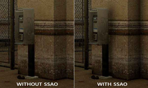
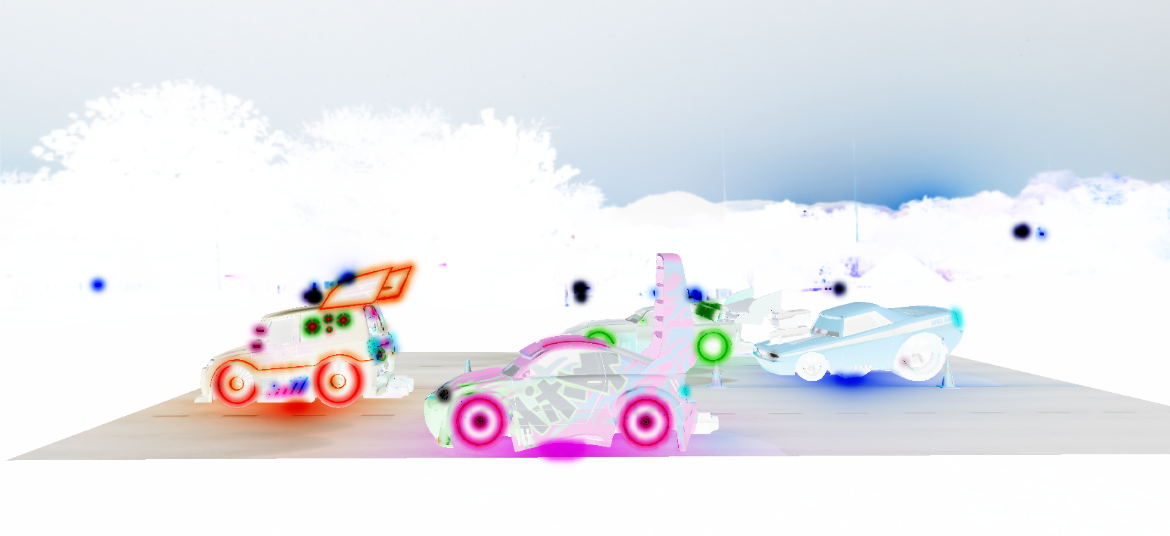
SSAO

To add some depth to the scene, I learned how to implement SSAO (Screen Space Ambient Occlusion). This technique simulates how ambient light is blocked by surrounding geometry. It creates contact shadows in corners, crevices, and especially under the car, which really helps “ground” the model. Here is an example below:

To simplify the implementation, I created a dedicated SSAO class. The rendering happens in two stages: a calculation pass (which generates the raw occlusion) and a blur pass (to clean up the noise).

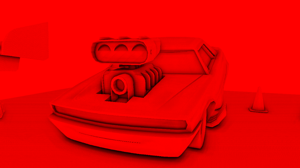
I configure the first step in SSAO::Init, which handles calling GenerateKernel and GenerateNoiseTexture. The calculation relies on statistical sampling. Instead of casting rays everywhere, I generate a Kernel (a hemisphere) of 64 samples oriented towards the Z-axis.

void SSAO::GenerateKernel()
{
    std::uniform_real_distribution<float> random_floats(0.0, 1.0);
    std::default_random_engine generator;

    for (int i = 0; i < 64; ++i)
    {
        glm::vec3 sample(
            random_floats(generator) * 2.0 - 1.0,
            random_floats(generator) * 2.0 - 1.0,
            random_floats(generator)
        );

        sample = glm::normalize(sample);
        sample *= random_floats(generator);

        float scale = static_cast<float>(i) / 64.0;
        scale = std::lerp(0.1f, 1.0f, scale * scale);
        sample *= scale;

        kernel_.push_back(sample);
    }
}

For the 4x4 noise texture, I generate it procedurally here, but you could totally use a simple noise image loaded from disk. The texture is set to GL_REPEAT so it tiles over the entire screen.

std::uniform_real_distribution<float> random_floats(0.0, 1.0);
std::default_random_engine generator;

std::vector<glm::vec4> ssao_noise;

for (unsigned int i = 0; i < 16; i++)
{
    glm::vec4 noise(
        random_floats(generator) * 2.0 - 1.0,
        random_floats(generator) * 2.0 - 1.0,
        0.0f,
        0.0f
    );
    ssao_noise.push_back(noise);
}

Once the Kernel and noise are ready to go, we move on to rendering.

But remember, the job isn’t done yet. The raw image is pretty much unusable because of the noise. That leaves us with the 2nd pass: the Blur.

In the render function, you can clearly see the sequence. After generating the occlusion, I immediately bind the blur pipeline (ssao_.Blur()) and redraw the Quad on top.

void SceneSample::RenderSSAOPass(const glm::mat4& view, const glm::mat4& projection)
{
    g_buffer_.BindTextures();
    
    ssao_.BeginGen(projection, view);
    quad_mesh_.Draw();
    ssao_.End();

    ssao_.Blur();
    quad_mesh_.Draw();
    ssao_.End();
}

The blur shader is super simple. Unlike a Gaussian blur (which we’ll see later), here a simple average does the trick (Box Blur). I iterate over a 4x4 texel grid around the current position, sum up the occlusion values, and divide the whole thing by 16.

vec2 texelSize = 1.0 / vec2(textureSize(ssaoInput, 0));
float result = 0.0;

for (int x = -2; x < 2; ++x)
{
    for (int y = -2; y < 2; ++y)
    {
        vec2 offset = vec2(float(x), float(y)) * texelSize;
        result += texture(ssaoInput, TexCoords + offset).r;
    }
}

FragColor = result / 16.0;

And here is the result: the noise is gone, giving way to soft and natural occlusion!

PBR Lighting

Once the G-Buffer and SSAO data are ready, we can finally calculate the lighting. This step is both cool to look at and a little bit more complex to wrap your head around, hehe…

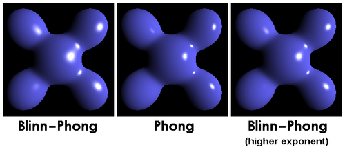
Initially, I implemented the 3 light types (Directional, Point, Spot) using the Blinn-Phong model. This is the “classic” approach: you add a Diffuse component (the object’s color) and a Specular component (the shiny reflection).

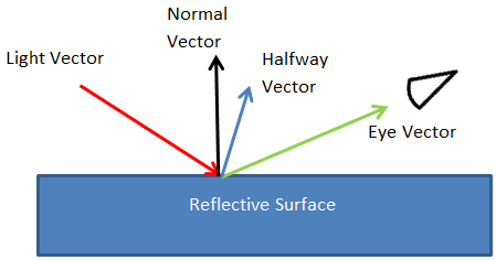
The Half-way Vector (a vector halfway between the view direction and the light direction) allows us to get the specular reflection much faster than doing a full physical reflection calculation.

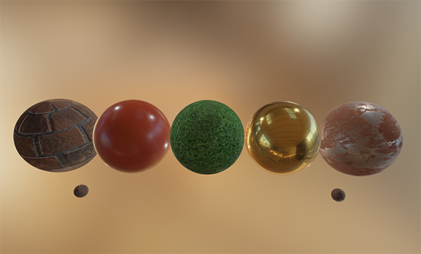
That’s already not bad, but physically speaking, it’s not very realistic. To get much more believable cars, I switched to PBR (Physically Based Rendering), which is a more modern rendering method.

To achieve this realism, PBR simulates the surface of objects at a microscopic level (Microfacets). Even if a surface looks smooth, under a microscope, it’s actually irregular. The “rougher” it is, the more chaotically the light scatters.

To control this, we ditch the old “Specular Maps” in favor of 3 physical textures:

• Albedo: The base color.
• Metallic: Is it metal or plastic/wood? (0.0 or 1.0).
• Roughness: The surface condition (Smooth or Rough).

I implemented a dedicated ARM texture (Ambient Occlusion, Roughness, Metallic). This allowed me to pack all three physical properties into the RGB channels of a single texture

float ao = useAOMap ? texture(aoMap, TexCoords).r : 1.0;
float roughness = useRoughnessMap ? texture(roughnessMap, TexCoords).r : 0.5;
float metallic = useMetallicMap ? texture(metallicMap, TexCoords).r : 0.0;

gARM = vec4(ao, roughness, metallic, 1.0);

With PBR, everything relies on the Reflectance Equation. It’s the mathematical formula that sums up all incoming light to calculate exactly how much is reflected back to the eye.

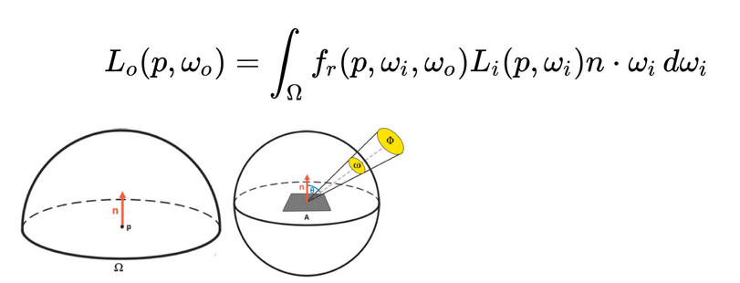
The most important term in this equation is the BRDF (fr). This determines how light reacts when it hits the surface. In my engine, I use the industry standard: the Cook-Torrance BRDF.

This model splits the light into two distinct parts:

• Diffuse (Lambert): The “color” part (internal refraction).
• Specular (Cook-Torrance): The “reflection” part (surface reflection).

The complete BRDF equation looks like this:

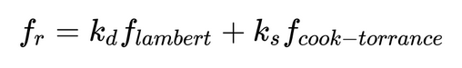
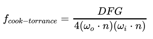
For the Diffuse part, it’s super simple: it’s just the color divided by PI (c / PI). The Specular part is more complex. It uses 3 physical functions (Distribution, Fresnel, Geometry) to simulate the microfacets. I won’t go into the math details here, but for the curious, everything is explained in depth on LearnOpenGL/PBR/Theory.

In the end, when we plug fr into the base equation, we get the full formula that my shader solves for every single light:

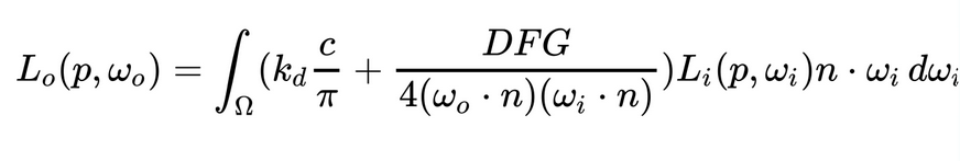
To translate this math into code, you can see the equation’s structure mirrored exactly in the lighting loop. We calculate the D, F, and G terms for the specular component, and we respect the conservation of energy by adjusting the diffuse (kD) based on the specular (kS).

Here is the snippet from the Fragment Shader that handles a light:

vec3 L = normalize(lights[i].position - fragPos);
vec3 V = normalize(viewPos - fragPos);
vec3 H = normalize(V + L); // Half-way vector

// (Cook-Torrance)
float NDF = DistributionGGX(N, H, roughness);   // D
float G   = GeometrySmith(N, V, L, roughness);
vec3  F   = fresnelSchlick(max(dot(H, V), 0.0), F0);

// Specular calculation
vec3 numerator    = NDF * G * F;
float denominator = 4.0 * max(dot(N, V), 0.0) * max(dot(N, L), 0.0);
vec3 specular     = numerator / denominator;

// Energy conservation
vec3 kS = F;
vec3 kD = vec3(1.0) - kS;
kD *= 1.0 - metallic; 

// Reflectance Equation
float NdotL = max(dot(N, L), 0.0);
Lo += (kD * albedo / PI + specular) * radiance * NdotL;

Light IBL

Okay, with that, we have the PBR basics. But we’re missing one essential thing to really make it pop. Right now, our Diffuse just boils down to c / PI, and metal doesn’t reflect anything at all.

This is where IBL (Image Based Lighting) comes in. The idea is to use the HDR Skybox as a giant light source. Instead of just having a point light at a specific position, we consider that every pixel of the sky emits light.

To solve the light integral with this infinite number of light sources, we start by simplifying the equation. We split the calculation into two distinct parts: the Diffuse and the Specular.

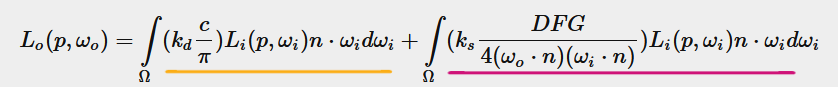
The yellow part represents the Diffuse integral, and the pink part the Specular one. By separating them, it allows us to first solve the Diffuse part (Irradiance) independently. You can see the mathematical details here LearnOpenGL/PBR/IBL/Diffuse-irradiance

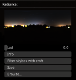
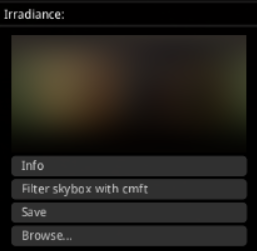
To make this equation work, we need 3 specific textures:

• Irradiance Map: A very blurry version of the skybox for diffuse light.
• Prefilter Map: The skybox stored with different blur levels in the mipmaps.
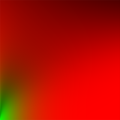
• BRDF LUT (Look Up Table): This is the famous “red and green” texture. It contains the pre-calculated Scale and Bias values of the BRDF.

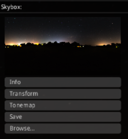
Calculating all of this in real-time would be way too heavy. So, I generated these textures Offline (in advance) using cmft Studio. I feed it my HDR Skybox, and it outputs the Irradiance and Prefilter .hdr files.

For the Diffuse, it’s straightforward: we sample from the Irradiance Map. For the Specular, that’s where we apply the Split Sum. We retrieve the light via textureLod and mix it all with the values from the LUT.

Once we have this full ambient lighting, we just add it to the direct lighting result (Lo) and the emissive.

// --- IBL DIFFUSE ---
vec2 uvIrradiance = SampleSphericalMap(N);
vec3 irradiance = texture(irradianceMap, uvIrradiance).rgb * skyboxIntensity;
vec3 diffuse = irradiance * albedo;

// --- IBL SPECULAR ---
const float MAX_REFLECTION_LOD = 8.0;
vec2 uvPrefilter = SampleSphericalMap(R);
vec3 prefilteredColor = textureLod(prefilterMap, uvPrefilter, roughness * MAX_REFLECTION_LOD).rgb;

vec2 brdf  = texture(brdfLUT, vec2(max(dot(N, V), 0.0), roughness)).rg;

vec3 specular = prefilteredColor * (F0 * brdf.x + brdf.y);
specular *= (1.0 - roughness);

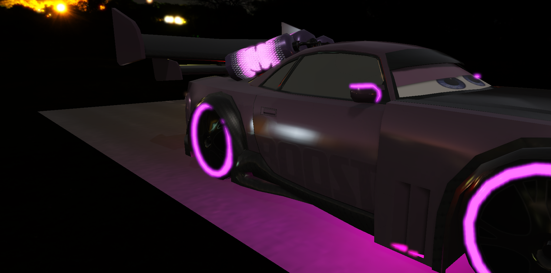
vec3 ambient = (kD * diffuse + specular) * ao;

And here is the final result on the car (Boost)

Framebuffer

To make Deferred Rendering, Post-Processing, or even IBL generation possible, I can’t draw directly to the screen (the Backbuffer). I need to draw “off-screen”. To avoid rewriting the OpenGL configuration every time, I use a common::Framebuffer abstraction. It automatically handles:

• Texture creation.
• Attaching to the Framebuffer Object (FBO).
• Depth/Stencil management.

The whole setup happens in common::Framebuffer::Load, where texture creation and especially the activation of MRT (Multiple Render Targets) is handled. This is what allows writing to gPosition, gNormal, and gAlbedo at the same time. It comes down to two calls:

glFramebufferTexture2D(GL_FRAMEBUFFER, GL_COLOR_ATTACHMENT0 + i, target, texture_id, 0);
glDrawBuffers(attachment_count, attachments_list.data());

Final step of the pipeline: rendering to a Screen Quad. Once all the geometry is calculated, instead of displaying the image directly, I project it onto a simple quad that covers the entire screen. I added several different filters (Grayscale, Inverse, Sharpen).

Normal

Grayscale

Inverse

Sharpen

HDR + Bloom

By default, a standard screen (LDR) and OpenGL clamp colors between 0.0 and 1.0. The problem is that with PBR, the sun or metallic reflections can have intensities of 10.0, 50.0, or more. If we clamp everything at 1.0, we lose all the nuance in the highlights.

I use a Framebuffer with a floating point color format (GL_RGBA16F). This allows the graphics card to store values well above 1.0 without losing them. In my HDRBuffer abstraction, I initialize this special buffer and enable MRT (Multiple Render Targets) to extract the brightness at the same time:

glTexImage2D(GL_TEXTURE_2D, 0, GL_RGBA16F, width, height, 0, GL_RGBA, GL_FLOAT, NULL);
constexpr unsigned int attachments[2] = { GL_COLOR_ATTACHMENT0, GL_COLOR_ATTACHMENT1 };
glDrawBuffers(2, attachments);

Since our screens physically cannot display a value of 10.0, we must convert the HDR image to LDR (0.0 - 1.0) at the very end of the pipeline. This is Tone Mapping. I use Exposure Tone Mapping.

Next, we must not forget Gamma Correction. Physical calculations are done in linear space, but we (human eye and screens) expect a Gamma curve (power 2.2).

// post_process.frag
void main()
{
    const float gamma = 2.2;
    vec3 hdrColor = texture(scene, TexCoords).rgb;

    vec3 result = vec3(1.0) - exp(-hdrColor * exposure);

    result = pow(result, vec3(1.0 / gamma));

    FragColor = vec4(result, 1.0);
}

Bloom is the glowing halo effect around very bright objects. It gives the illusion that the light is so strong it “bleeds” into the camera.

To achieve bloom, I do it in 3 steps:

1. In the main PBR shader, while rendering the scene, we separate pixels that exceed a certain brightness (Threshold).

// deferred_lit.frag
FragColor = vec4(result, 1.0);

float brightness = dot(result, vec3(0.2126, 0.7152, 0.0722));
BrightColor = brightness > 1.0 ? vec4(result, 1.0) : vec4(0.0, 0.0, 0.0, 1.0);

2. Add Gaussian Blur: I take the “BrightColor” texture and blur it heavily. To optimize, instead of doing one massive blur in a single go, I use Ping-Pong Rendering: I blur horizontally, then vertically, multiple times in succession. This is managed by my Bloom class which alternates between two Framebuffers:

// graphics::Bloom::RenderBloom
bool horizontal = true;
for (int i = 0; i < amount; i++)
{
    glBindFramebuffer(GL_FRAMEBUFFER, pingpongFBO_[horizontal]);
    blur_pipeline_.SetBool("horizontal", horizontal);

    quadMesh.Draw();

    horizontal = !horizontal;
}

3. Combination Finally, in the final post-process shader, we simply add the original HDR image with the blurred image (Bloom). This is where it all comes together.

// post_process.frag
vec3 hdrColor = texture(scene, TexCoords).rgb;
vec3 bloomColor = texture(bloomBlur, TexCoords).rgb;

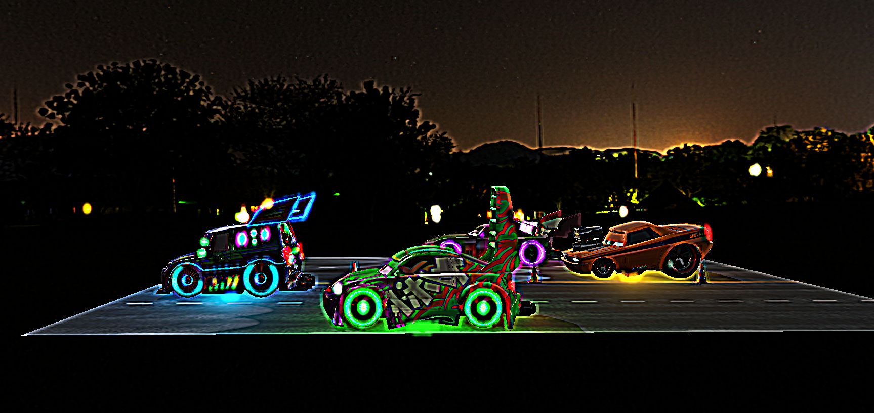
hdrColor += bloomColor; 

Now let’s compare the result without and with bloom!

Bloom OFF

Bloom ON

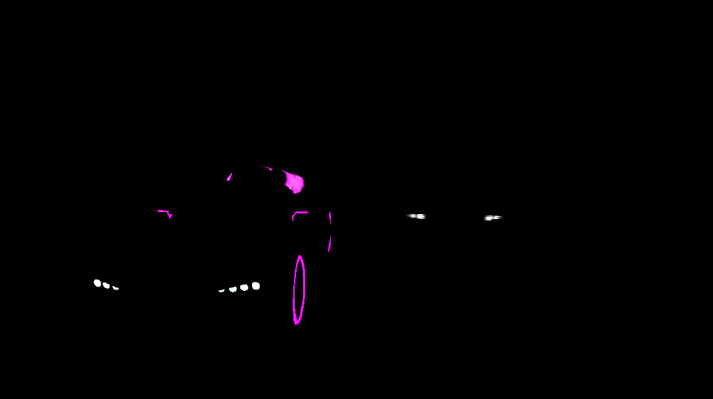
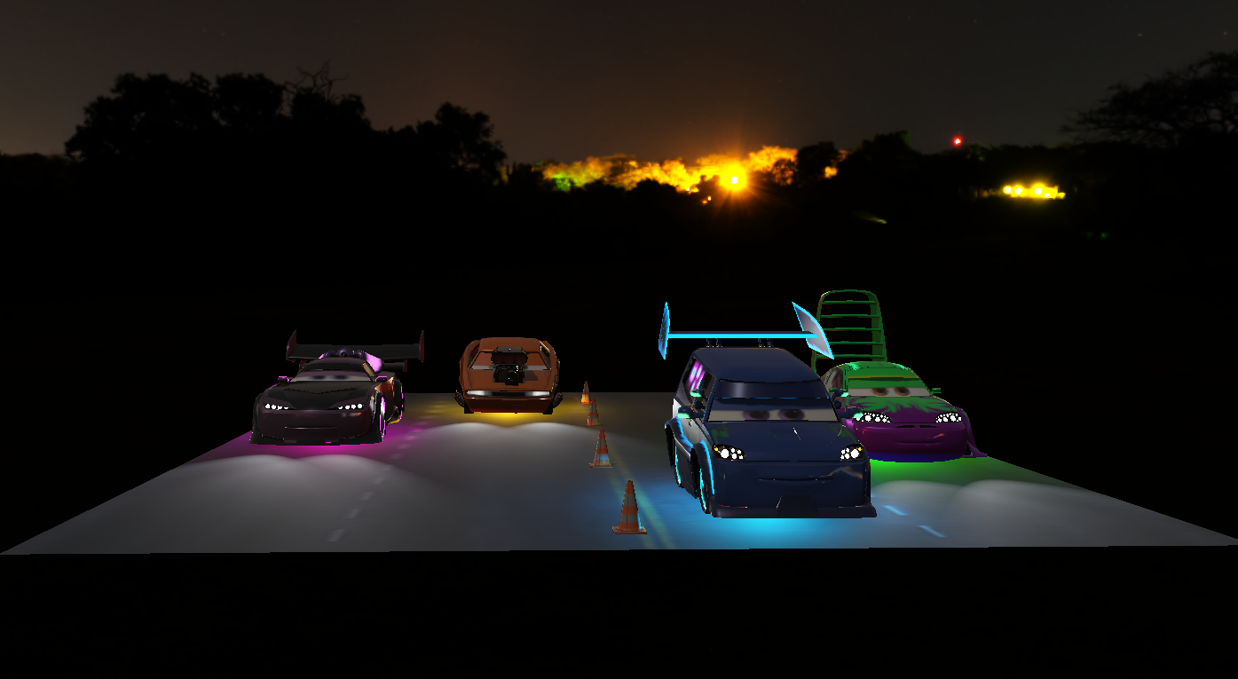
Emission

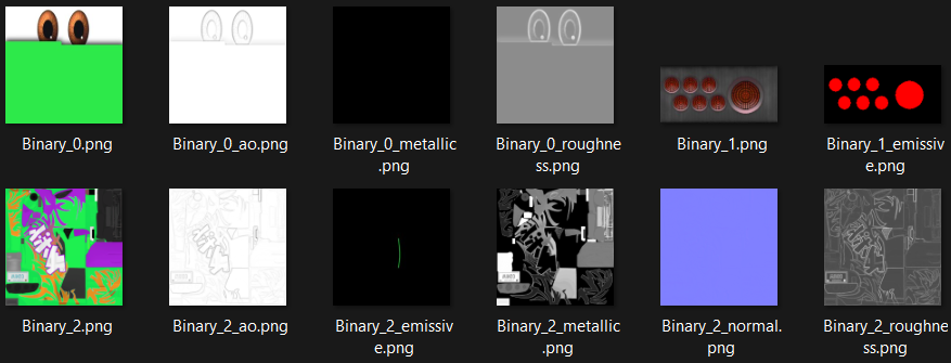
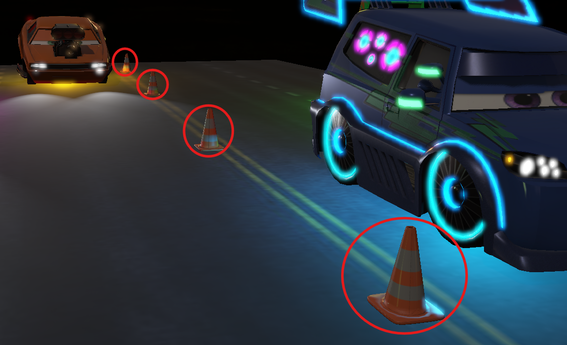
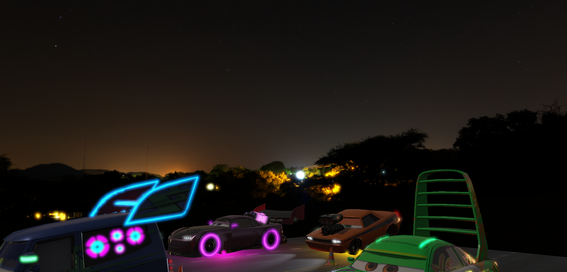
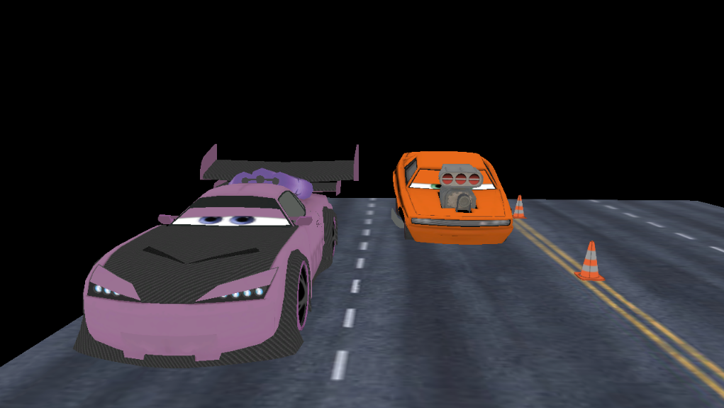
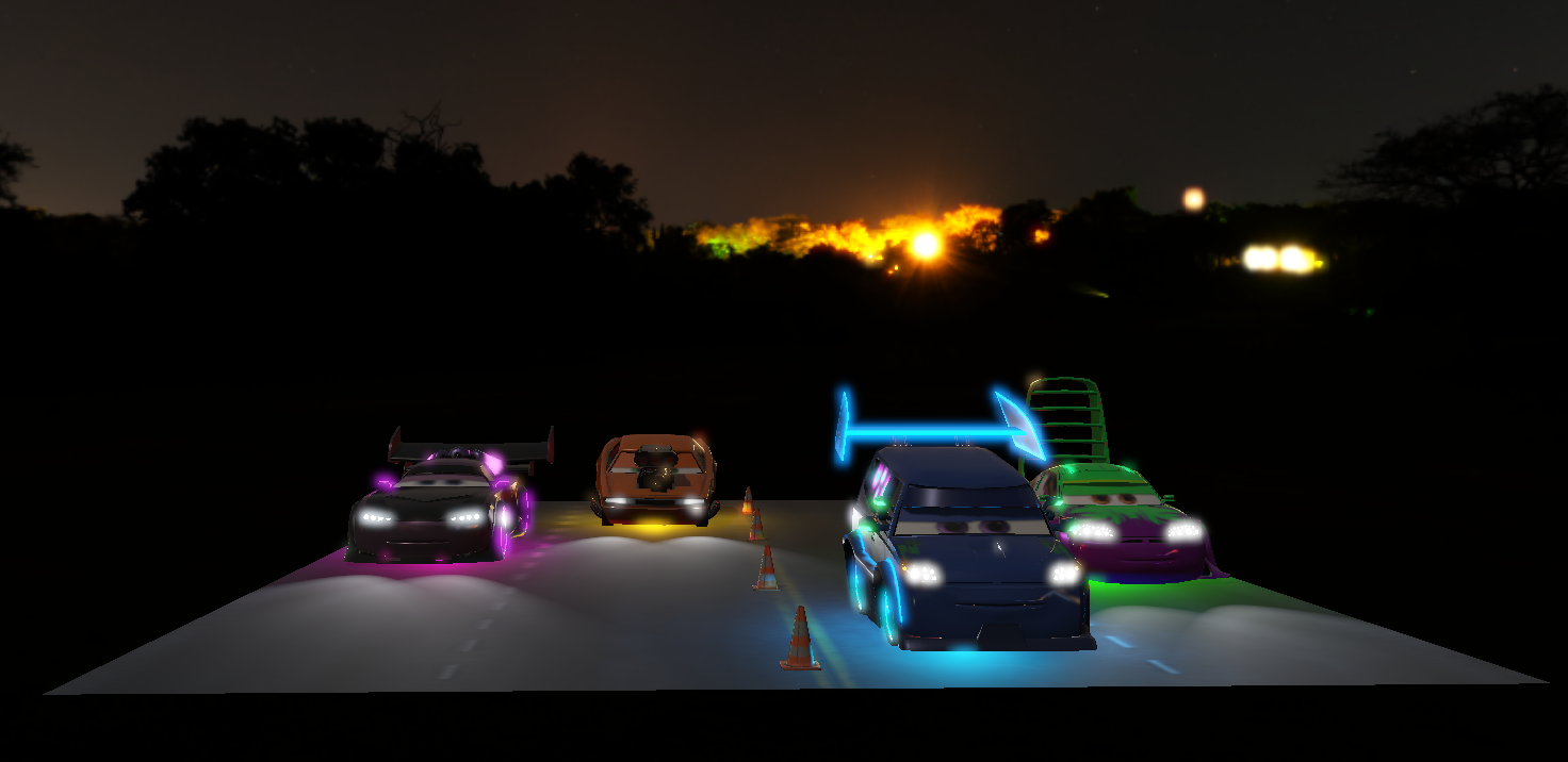
A small bonus: I added Emission to my models. This allows certain parts of the object to “glow” in the dark like neon lights, to really fit the scene in Cars.

The integration was honestly simple. On the loading side (Assimp), I just had to retrieve the corresponding texture:

LoadTex(aiTextureType_EMISSIVE, m.emissiveMap);

Next, I store it in my G-Buffer. I multiply the color by an emissiveStrength to be able to control the intensity of the “glow”:

// gbuffer.frag
gEmissive = useEmissiveMap ? texture(emissiveMap, TexCoords).rgb * emissiveStrength : vec3(0.0);

And finally, in the deferred lighting pass (deferred_lit.frag), it acts as pure light. So I simply add it to the final result, without any shadow calculation. This is where Bloom does all the work: since the intensity is high, the brightness calculation will capture these pixels and create the glowing halo.

// deferred_lit.frag
vec3 emissive = texture(gEmissive, TexCoords).rgb;

// Adding emission
vec3 result = ambient + Lo + emissive;

FragColor = vec4(result, 1.0);

float brightness = dot(result, vec3(0.2126, 0.7152, 0.0722));
BrightColor = brightness > 1.0 ? vec4(result, 1.0) : vec4(0.0, 0.0, 0.0, 1.0);

Here is an emissive map I made myself for the DJ car (the blue one) which took me 2.5 hours to make (really).

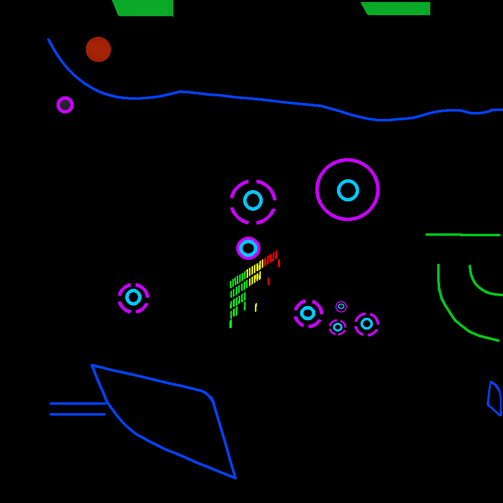
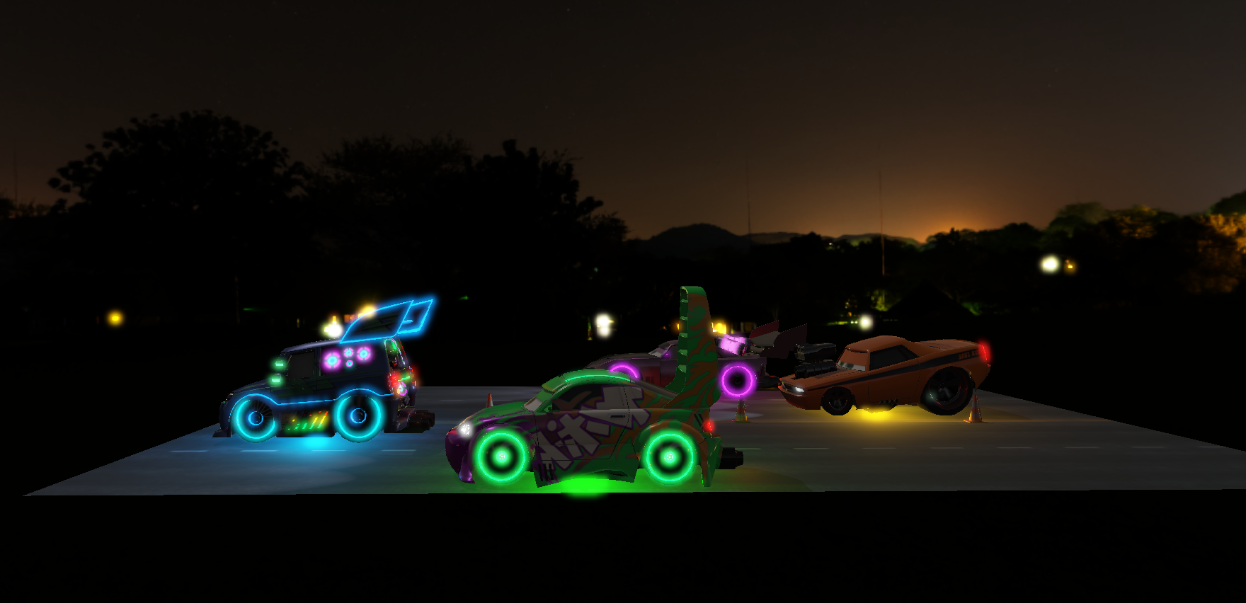
Then the final result which I am proud of!

Conclusion

That’s it! We’ve pretty much covered all the techniques used in my final 3D scene. Throughout this module, I had quite a few moments of confusion because I’m not used to working at such a low level with the GPU, but little by little, you get used to it. I also got to see how the GPU can be used for calculations other than pure rendering (via CUDA).

It was both frustrating and rewarding to see a working result. Personally, I found it very interesting to dive into OpenGL. I learned a lot of things that helped me better understand how graphics engines work, even though today’s big engines tend to use DX11, DX12, or Vulkan.

The experience was cool! Trying to create a small scene themed after Cars is what motivated me the most in this module. If something is missing from my scene, it would be shadows for Point Lights and maybe Cascaded Shadow Mapping. But overall, I remain very proud of this 3D scene! Now, whenever I play any AAA game, I’ll always notice the techniques I learned here.

Feel free to check out my Github to see the implementation in more detail.

With that, thanks for reading!